harmonic mean chi-squared test

p-values and confidence intervals from the harmonic mean chi-squared test.

hMeanChiSq(
  z,
  w = rep(1, length(z)),
  alternative = c("greater", "less", "two.sided", "none"),
  bound = FALSE
)

hMeanChiSqMu(
  thetahat,
  se,
  w = rep(1, length(thetahat)),
  mu = 0,
  alternative = c("greater", "less", "two.sided", "none"),
  bound = FALSE
)

hMeanChiSqCI(
  thetahat,
  se,
  w = rep(1, length(thetahat)),
  alternative = c("two.sided", "greater", "less", "none"),
  conf.level = 0.95
)

Arguments

z

Numeric vector of z-values.

w

Numeric vector of weights.

alternative

Either "greater" (default), "less", "two.sided", or "none". Specifies the alternative to be considered in the computation of the p-value.

bound

If FALSE (default), p-values that cannot be computed are reported as NaN. If TRUE, they are reported as "> bound".

thetahat

Numeric vector of parameter estimates.

se

Numeric vector of standard errors.

mu

The null hypothesis value. Defaults to 0.

conf.level

Numeric vector specifying the conf.level of the confidence interval. Defaults to 0.95. summarize the gamma values, i.e., the local minima of the p-value function between the thetahats. Defaults is a vector of 1s.

Value

hMeanChiSq: returns the p-values from the harmonic mean chi-squared test based on the study-specific z-values.

hMeanChiSqMu: returns the p-value from the harmonic mean chi-squared test based on study-specific estimates and standard errors.

hMeanChiSqCI: returns a list containing confidence interval(s) obtained by inverting the harmonic mean chi-squared test based on study-specific estimates and standard errors. The list contains:

CI

Confidence interval(s).

If the alternative is "none", the list also contains:

gamma

Local minima of the p-value function between the thetahats.

References

Held, L. (2020). The harmonic mean chi-squared test to substantiate scientific findings. Journal of the Royal Statistical Society: Series C (Applied Statistics), 69, 697-708. doi:10.1111/rssc.12410

Author

Leonhard Held, Florian Gerber

Examples

## Example from Fisher (1999) as discussed in Held (2020)
pvalues <- c(0.0245, 0.1305, 0.00025, 0.2575, 0.128)
lower <- c(0.04, 0.21, 0.12, 0.07, 0.41)
upper <- c(1.14, 1.54, 0.60, 3.75, 1.27)
se <- ci2se(lower = lower, upper = upper, ratio = TRUE)
thetahat <- ci2estimate(lower = lower, upper = upper, ratio = TRUE)

## hMeanChiSq() --------
hMeanChiSq(z = p2z(p = pvalues, alternative = "less"),
           alternative = "less")
#> [1] 0.0004840125
hMeanChiSq(z = p2z(p = pvalues, alternative = "less"),
           alternative = "two.sided")
#> [1] 0.000968025
hMeanChiSq(z = p2z(p = pvalues, alternative = "less"),
           alternative = "none")
#> [1] 0.0154884

hMeanChiSq(z = p2z(p = pvalues, alternative = "less"),
           w = 1 / se^2, alternative = "less")
#> [1] 0.0003410182
hMeanChiSq(z = p2z(p = pvalues, alternative = "less"),
           w = 1 / se^2, alternative = "two.sided")
#> [1] 0.0006820365
hMeanChiSq(z = p2z(p = pvalues, alternative = "less"),
           w = 1 / se^2, alternative = "none")
#> [1] 0.01091258


## hMeanChiSqMu() --------
hMeanChiSqMu(thetahat = thetahat, se = se, alternative = "two.sided")
#> [1] 0.0009954952
hMeanChiSqMu(thetahat = thetahat, se = se, w = 1 / se^2,
             alternative = "two.sided")
#> [1] 0.000723444
hMeanChiSqMu(thetahat = thetahat, se = se, alternative = "two.sided",
             mu = -0.1)
#> [1] 0.003089007

## hMeanChiSqCI() --------
## two-sided
CI1 <- hMeanChiSqCI(thetahat = thetahat, se = se, w = 1 / se^2,
                    alternative = "two.sided")
CI2 <- hMeanChiSqCI(thetahat = thetahat, se = se, w = 1 / se^2,
                    alternative = "two.sided", conf.level = 0.99875)
## one-sided
CI1b <- hMeanChiSqCI(thetahat = thetahat, se = se, w = 1 / se^2,
                     alternative = "less", conf.level = 0.975)
CI2b <- hMeanChiSqCI(thetahat = thetahat, se = se, w = 1 / se^2,
                     alternative = "less", conf.level = 1 - 0.025^2)

## confidence intervals on hazard ratio scale
print(exp(CI1$CI), digits = 2)
#>      lower upper
#> [1,]  0.21  0.74
print(exp(CI2$CI), digits = 2)
#>      lower upper
#> [1,]  0.16  0.97
print(exp(CI1b$CI), digits = 2)
#>      lower upper
#> [1,]     0  0.74
print(exp(CI2b$CI), digits = 2)
#>      lower upper
#> [1,]     0  0.97


## example with confidence region consisting of disjunct intervals
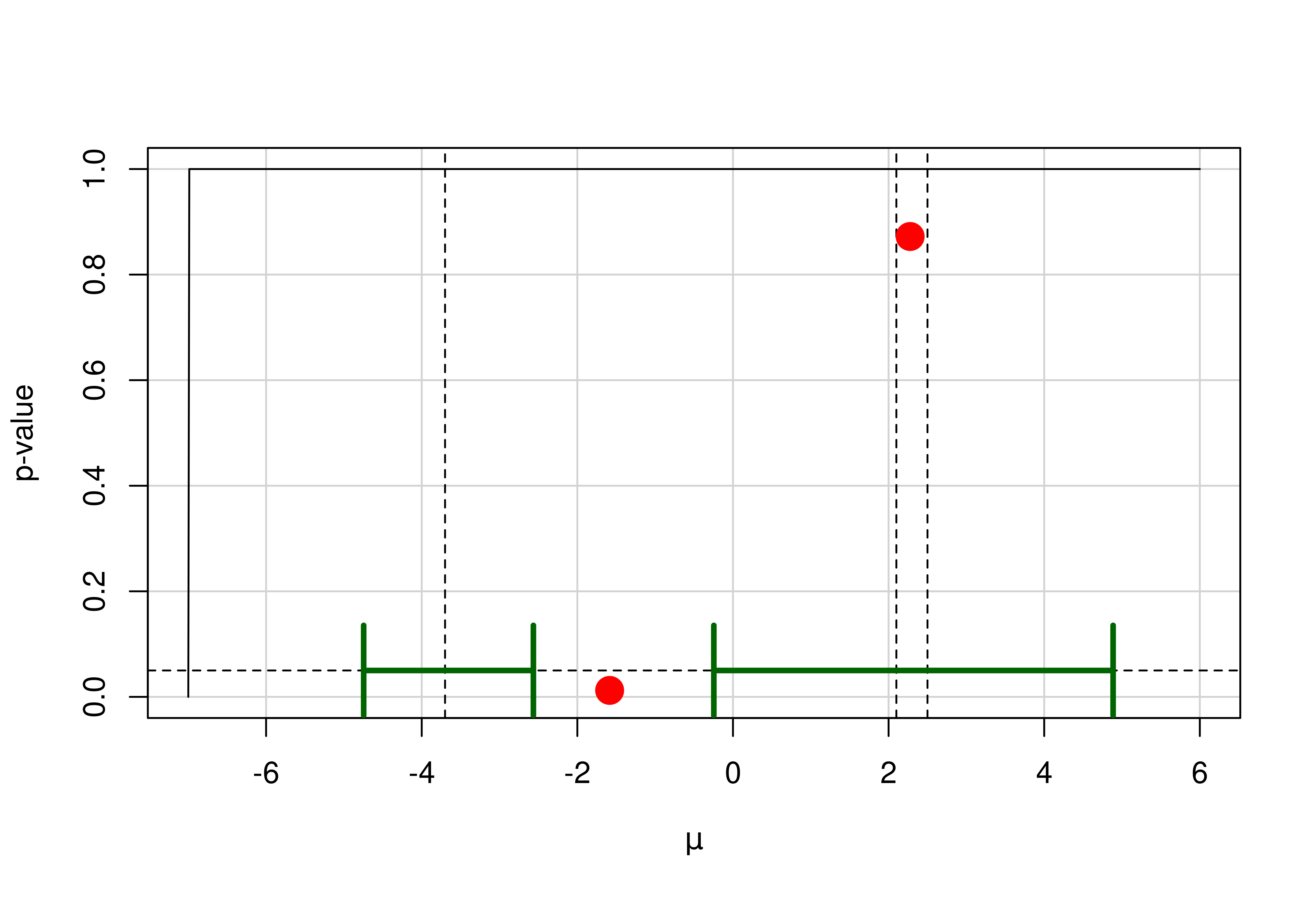
thetahat2 <- c(-3.7, 2.1, 2.5)
se2 <- c(1.5, 2.2, 3.1)
conf.level <- 0.95; alpha <- 1 - conf.level
muSeq <- seq(-7, 6, length.out = 1000)
pValueSeq <- hMeanChiSqMu(thetahat = thetahat2, se = se2,
                          alternative = "none", mu = muSeq)
(hm <- hMeanChiSqCI(thetahat = thetahat2, se = se2, alternative = "none"))
#> $CI
#>           lower     upper
#> [1,] -4.7459650 -2.564739
#> [2,] -0.2457423  4.885610
#> 
#> $gamma
#>        minimum pvalue_fun/gamma
#> [1,] -1.584762       0.01227696
#> [2,]  2.277232       0.87220092
#> 

plot(x = muSeq, y = pValueSeq, type = "l", panel.first = grid(lty = 1),
     xlab = expression(mu), ylab = "p-value")
abline(v = thetahat2, h = alpha, lty = 2)
arrows(x0 = hm$CI[, 1], x1 = hm$CI[, 2], y0 = alpha,
       y1 = alpha, col = "darkgreen", lwd = 3, angle = 90, code = 3)
points(hm$gamma, col = "red", pch = 19, cex = 2)