Prediction interval for effect estimate of replication study — predictionInterval • ReplicationSuccess

Computes a prediction interval for the effect estimate of the replication study.

predictionInterval(
  thetao,
  seo,
  ser,
  tau = 0,
  conf.level = 0.95,
  designPrior = "predictive"
)

Arguments

thetao: Numeric vector of effect estimates from original studies.
seo: Numeric vector of standard errors of the original effect estimates.
ser: Numeric vector of standard errors of the replication effect estimates.
tau: Between-study heterogeneity standard error. Default is 0 (no heterogeneity). Is only taken into account when designPrior is "predictive" or "EB".
conf.level: The confidence level of the prediction intervals. Default is 0.95.
designPrior: Either "predictive" (default), "conditional", or "EB". If "EB", the contribution of the original study to the predictive distribution is shrunken towards zero based on the evidence in the original study (with empirical Bayes).

Value

A data frame with the following columns

lower: Lower limit of prediction interval,
mean: Mean of predictive distribution,
upper: Upper limit of prediction interval.

Details

This function computes a prediction interval and a mean estimate under a specified predictive distribution of the replication effect estimate. Setting designPrior = "conditional" is not recommended since this ignores the uncertainty of the original effect estimate. See Patil, Peng, and Leek (2016) and Pawel and Held (2020) for details.

predictionInterval is the vectorized version of .predictionInterval_. Vectorize is used to vectorize the function.

References

Patil, P., Peng, R. D., Leek, J. T. (2016). What should researchers expect when they replicate studies? A statistical view of replicability in psychological science. Perspectives on Psychological Science, 11, 539-544. doi:10.1177/1745691616646366

Pawel, S., Held, L. (2020). Probabilistic forecasting of replication studies. PLoS ONE. 15, e0231416. doi:10.1371/journal.pone.0231416

Author

Samuel Pawel

Examples

predictionInterval(thetao = c(1.5, 2, 5), seo = 1, ser = 0.5, designPrior = "EB")
#>        lower      mean    upper
#> 1 -0.9257882 0.8333333 2.592455
#> 2 -0.4599640 1.5000000 3.459964
#> 3  2.6440396 4.8000000 6.955960

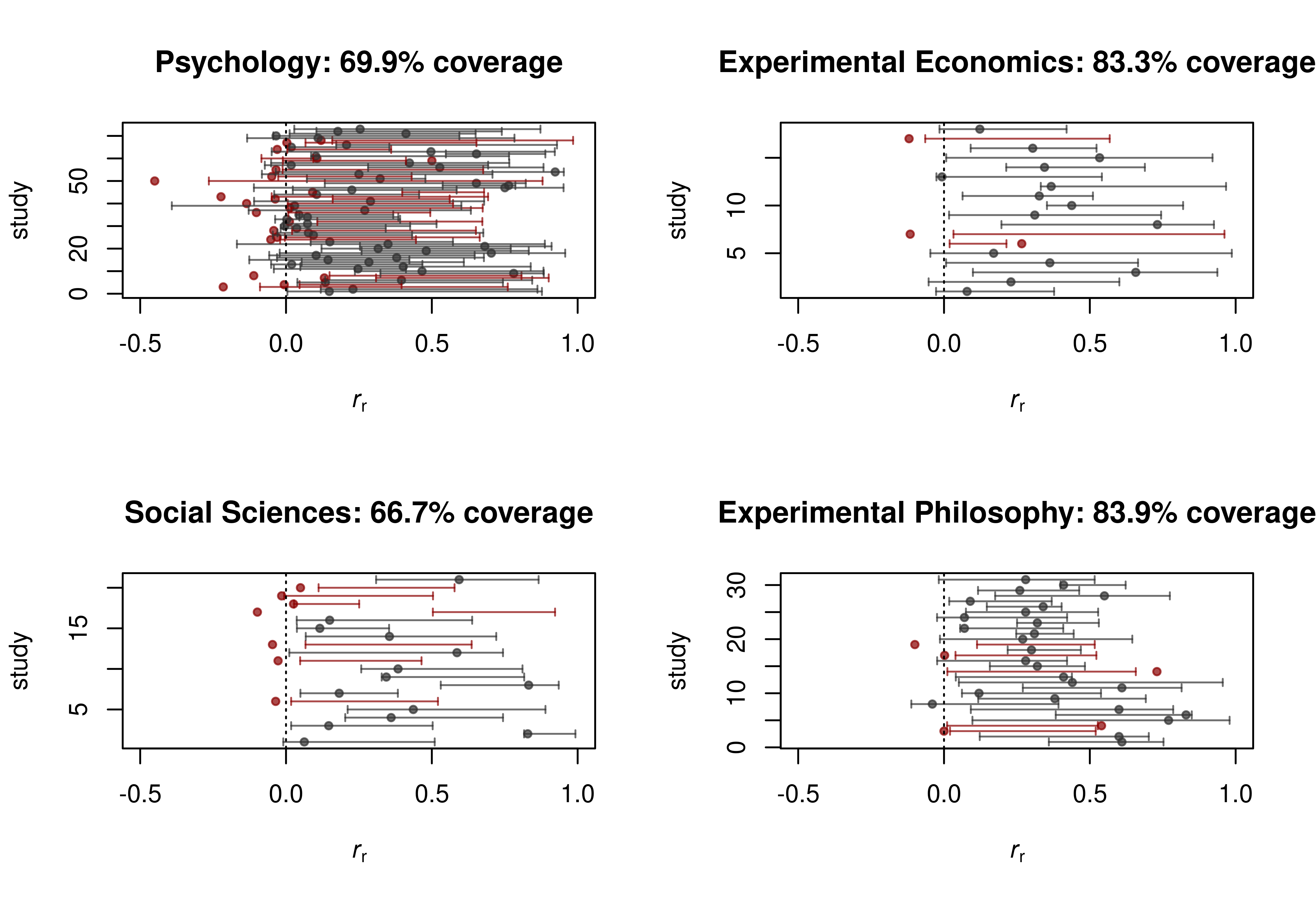
# compute prediction intervals for replication projects
data("RProjects", package = "ReplicationSuccess")
parOld <- par(mfrow = c(2, 2))
for (p in unique(RProjects$project)) {
  data_project <- subset(RProjects, project == p)
  PI <- predictionInterval(thetao = data_project$fiso, seo = data_project$se_fiso,
                           ser = data_project$se_fisr)
  PI <- tanh(PI) # transforming back to correlation scale
  within <- (data_project$rr < PI$upper) & (data_project$rr > PI$lower)
  coverage <- mean(within)
  color <- ifelse(within == TRUE, "#333333B3", "#8B0000B3")
  study <- seq(1, nrow(data_project))
  plot(data_project$rr, study, col = color, pch = 20,
       xlim = c(-0.5, 1), xlab = expression(italic(r)[r]),
       main = paste0(p, ": ", round(coverage*100, 1), "% coverage"))
  arrows(PI$lower, study, PI$upper, study, length = 0.02, angle = 90,
         code = 3, col = color)
  abline(v = 0, lty = 3)
}

par(parOld)